From Sensors to 3D Reconstruction of Urban Flow and Pollutant Fields

Urban flow and pollutant dispersion in dense city environments are shaped by the interaction between buildings, street canyons, wake regions, and local recirculation zones. These effects create complex spatial patterns that can be accurately resolved using high-fidelity CFD simulations. However, such simulations also produce very large datasets, making storage, post-processing, and repeated analysis computationally expensive.

To address this, low-cost reconstruction methods are developed to recover full urban flow and pollutant fields from a reduced set of sensor locations. The aim is to retain the main physical structures of the original CFD solution while significantly reducing the amount of data required for reconstruction.

We organize the work into two complementary methods:

Low-cost SVD reconstruction
Matrix-based reconstruction of the full 3D field from sparse sensor measurements.
Low-cost HOSVD reconstruction
Tensor-based reconstruction that preserves the spatial structure of the urban domain.

Together, these methods provide a path from sparse sensors to full-field reconstruction of velocity, pressure, turbulence quantities, and pollutant concentrations.

Methodology

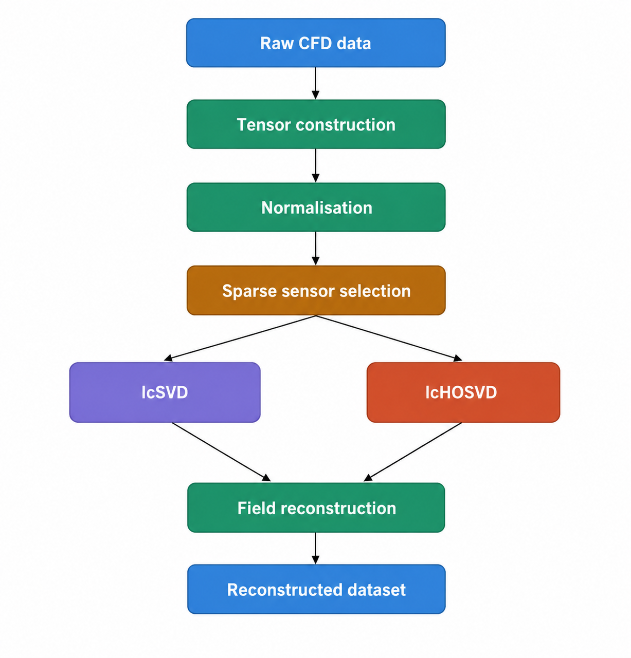
The reconstruction workflow starts from a high-fidelity CFD dataset. The full 3D field is sampled at a reduced number of sensor locations, and these sparse measurements are used to build a low-cost reduced-order representation. The reconstructed solution is then recovered over the complete computational domain.

Methodology for sparse-sensor 3D reconstruction

Methodology for reconstructing full 3D urban flow and pollutant fields from sparse sensor information.

The pipeline follows four main steps:

Full CFD field preparation
The original simulation data are arranged as spatial fields or tensors containing the variables of interest.
Sparse sensor selection
A reduced set of sensor locations is selected from the full computational domain.
Low-cost modal decomposition
The sparse dataset is decomposed using either lcSVD or lcHOSVD.
Full-field reconstruction
The reduced representation is expanded back to the full domain to recover the 3D flow or pollutant field.

Method 1: Low-Cost SVD Reconstruction

The first method is based on singular value decomposition. The original 3D field is unfolded into a two-dimensional matrix, where the spatial information is arranged along one dimension and the variables or snapshots are arranged along the other.

A reduced matrix is then built using only the selected sensor locations. Singular value decomposition is applied to this reduced matrix to extract the dominant spatial patterns of the flow or pollutant field.

Each retained SVD mode represents a global spatial structure of the field. The reconstructed solution is obtained by using a small number of these modes.

Main Features

lcSVD uses a matrix representation of the CFD field.
Only one SVD is required.
The method is computationally fast.
Each mode represents one global spatial pattern.
It is suitable when the dominant structures can be captured with a limited number of modes.

Because of its low computational cost, lcSVD is useful for rapid reconstruction and fast post-processing of large urban flow datasets.

Method 2: Low-Cost HOSVD Reconstruction

The second method is based on higher-order singular value decomposition. Unlike lcSVD, the lcHOSVD approach keeps the natural tensor structure of the 3D field.

Instead of unfolding the full domain into a single matrix, the decomposition is performed along the spatial directions separately. The reconstructed field is represented using directional modes in the x, y, and z directions, together with a compact core tensor.

Main Features

lcHOSVD preserves the tensor form of the 3D field.
The decomposition is performed separately along the spatial directions.
The core tensor stores the interaction between directional modes.
The method can capture richer three-dimensional structures.
It is useful for complex flows with directional dependencies and localized features.

Compared with lcSVD, lcHOSVD generally requires more computational work, but it can provide a more structured and accurate representation of complex 3D urban flow fields.

Low-cost SVD & HOSVD reconstruction scheme

lcSVD and lcHOSVD reconstruction strategy.

Sensor-Based Reconstruction

The sensor grid is selected to provide a reduced but representative sampling of the full domain. The number and distribution of sensors control the balance between cost and reconstruction accuracy.

Sparse sensor distribution

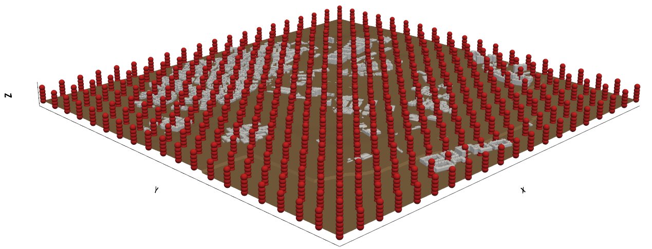
Example of sparse sensor locations used to construct the reduced dataset for low-cost reconstruction.

A denser sensor grid usually improves the reconstruction because more spatial information is available. However, the objective of the low-cost approach is to keep the number of sensors as small as possible while still preserving the main flow and pollutant structures. In this work, the decomposition was applied to two datasets and only 1-4% of the total spatial locations were used as sensors (Compression = 150x & 25x). The first dataset corresponds to a realistic urban-flow case from Vallecas, where the reconstruction is performed over a large computational domain containing several buildings and pollutant fields. The second dataset is a two-building LES case, used to test the methods on a more controlled flow with strong wake interactions and coherent vortical structures.

Ground Truth and Reconstructed Fields

The reconstruction quality is assessed by comparing the original CFD field with the reconstructed solutions. Representative results are shown for turbulent kinetic energy (k) and carbon monoxide (CO), which are selected from the Vallecas test case to illustrate the behaviour of the low-cost methods for both flow-related and pollutant-concentration fields.

Ground truth comparison k

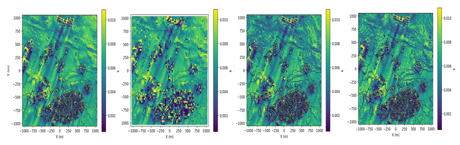
Comparison between ground truth, low-cost input and reconstructed fields using HOSVD and SVD, along with their low-cost counterparts for Turbulent Kinetic Energy (k).

Ground truth comparison CO

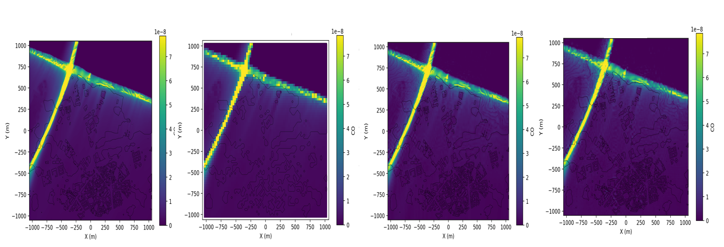
Comparison between ground truth, low-cost input and reconstructed fields using HOSVD and SVD, along with their low-cost counterparts for carbon monoxide (CO).

The comparison shows how the low-cost methods recover the main spatial distribution of the field while using only sparse sensor information. lcSVD provides a fast reconstruction based on global modes, while lcHOSVD gives a more structured tensor representation of the 3D field.

Flow-Structure Comparison

Beyond pointwise error, the reconstructed fields are also evaluated using flow-structure indicators. This helps assess whether the reduced reconstruction preserves coherent vortices, recirculation regions, and wake structures around buildings.

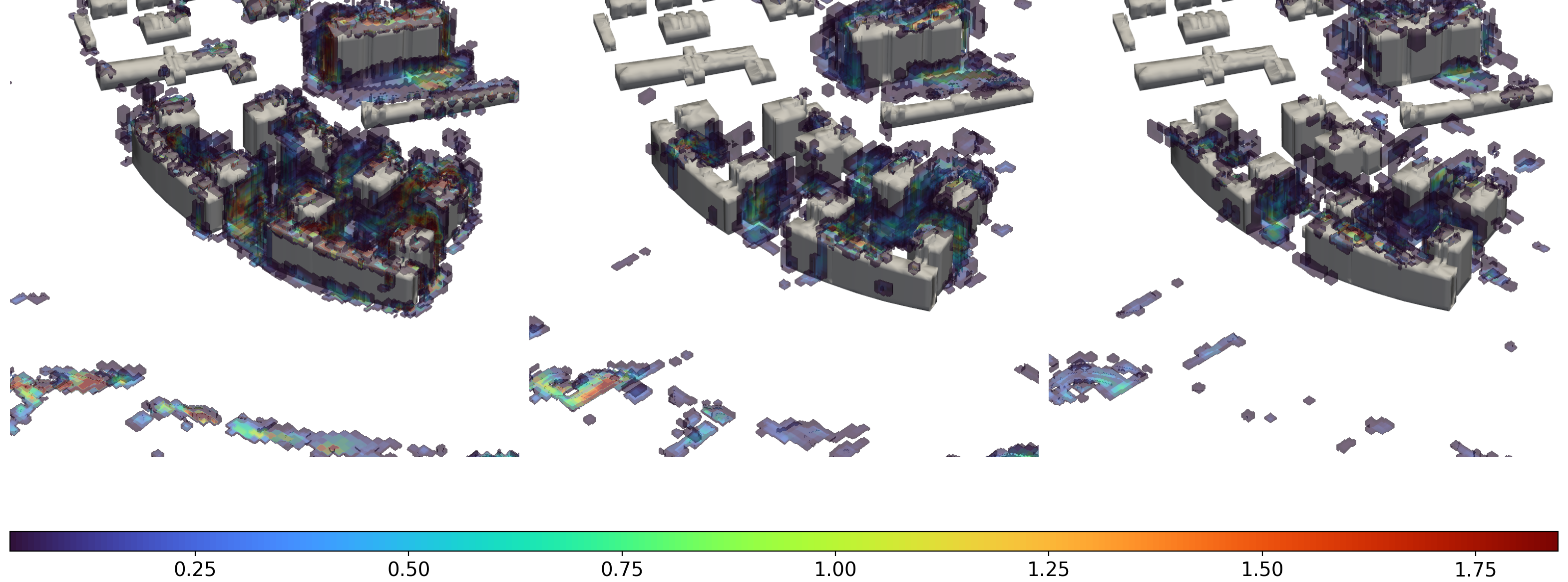
Q-criterion comparison for original and reconstructed fields

Q-criterion comparison of the ground truth with lcSVD and lcHOSVD.

Such comparisons are important because a low numerical error does not always guarantee that the relevant physical structures are preserved. For urban applications, retaining the main flow topology is essential for pollutant transport, ventilation studies, and sensor-informed analysis.

lcSVD and lcHOSVD Comparison

The two methods follow the same low-cost philosophy, but they behave differently.

lcSVD is faster because it applies a single SVD to a reduced matrix. It stores the field using a small number of global modes, which makes it attractive for rapid reconstruction and fast visualization.

lcHOSVD is more structured because it separates the spatial directions and stores their interaction through a core tensor. This usually improves the reconstruction of complex urban flow fields, especially when the field contains localized vortices, sharp gradients, or directional dependencies.

The trade-off between accuracy and computational cost is observed in both datasets. For the Vallecas urban-flow dataset, lcHOSVD gives lower reconstruction errors for all variables, with RRMSE values ranging from 4.63% to 34.91% for different variables. The corresponding lcSVD values range from 5.38% to 39.22%. However, lcSVD is significantly faster, reaching speed-ups of approximately 51× to 73×, compared with 3.6× to 4.0× for lcHOSVD.

For the two-building LES dataset, the comparison is made relative to the HOSVD reconstruction. In this case, lcHOSVD increases the RRMSE by only 0.28%, 2.82%, and 1.37% for the (u), (v), and (w) velocity components, respectively. The corresponding lcSVD increases are 1.47%, 8.84%, and 10.54%. This shows that lcHOSVD preserves the transverse and vertical flow structures more accurately, while lcSVD remains much faster, with an average speed-up of about 31×, compared with about 2.4× for lcHOSVD.

Dataset	Method	Error	Speed-up
Vallecas urban-flow dataset	lcHOSVD	4.63%–34.91% (RRMSE)	3.6×–4.0×
Vallecas urban-flow dataset	lcSVD	5.38%–39.22% (RRMSE)	51×–73×
Two-building LES dataset	lcHOSVD	0.28%–2.82% (ΔRRMSE)	≈2.4×
Two-building LES dataset	lcSVD	1.47%–10.54% (ΔRRMSE)	≈31×

In simple terms, lcSVD is usually faster, while lcHOSVD is usually more accurate for complex urban flow fields. This behaviour is more evident in the turbulent two-building test case, where the flow contains strong wake interactions, recirculation zones, and localized vortical structures between and downstream of the buildings.

In this case, the Q-criterion comparison shows that lcHOSVD preserves the main coherent structures more clearly, while lcSVD provides a faster but more globally smoothed reconstruction. The difference becomes visible around the near-building wake region, where the tensor structure used by lcHOSVD helps retain directional spatial interactions.

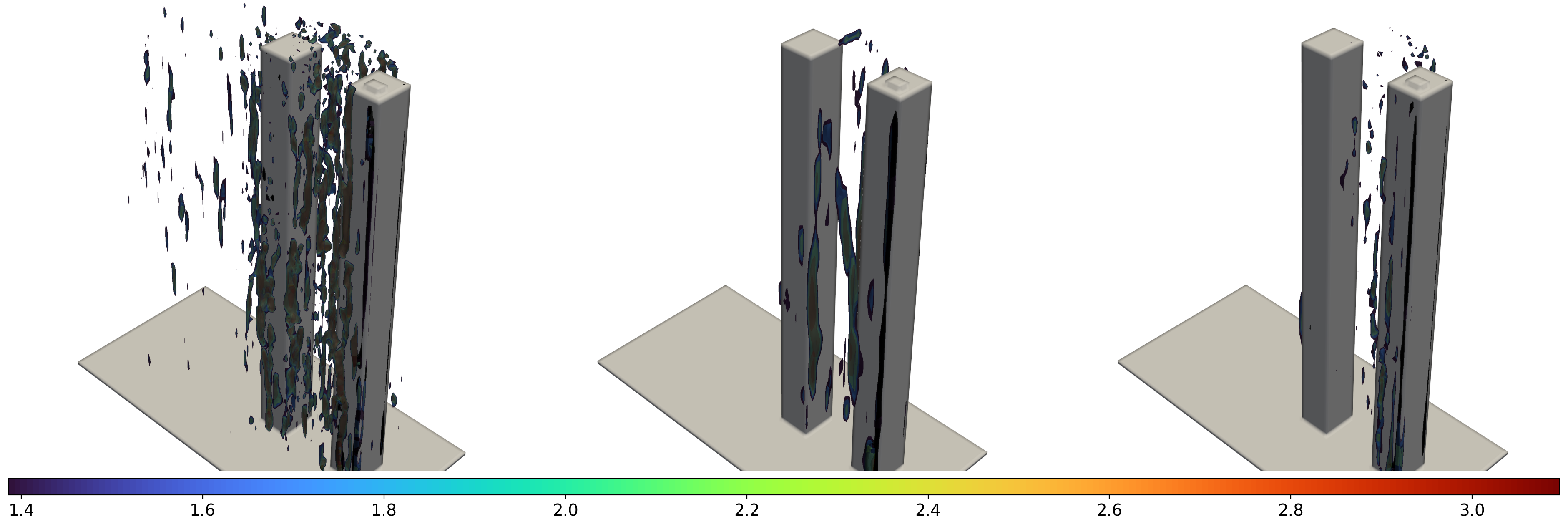
Q-criterion comparison for the two-building reconstruction case

Q-criterion comparison for the two-building LES case.

Applications

These methods can support:

3D urban wind-field reconstruction;
pollutant concentration reconstruction;
low-cost post-processing of CFD simulations;
sensor-informed urban digital twins;
rapid visualization of flow and pollutant fields;
reduced-order modelling for large urban datasets;
fast comparison of different urban flow scenarios.

Code and Data Availability

Code and tutorials: coming soon.
Data: coming soon.

References

Arindam Sengupta, Soledad Le Clainche, and collaborators.
Low-Cost Reconstruction of Three-Dimensional Urban Flow and Pollutant Fields from Sparse Sensors.
Manuscript in preparation.