ROMIA User Guide: Practical Workflow for CFD Acceleration
Steady-state CFD simulations often spend a large fraction of their total computational cost in the final convergence stage. At that point, the dominant flow topology is already established, but the solver still needs many additional iterations to relax the residuals and stabilize the engineering quantities of interest. This behaviour is especially relevant in industrial RANS simulations, where meshes may contain millions of cells and production runs can require hours or days on parallel clusters.
ROMIA — Reduced Order Model for Industrial Acceleration — is a non-intrusive reduced-order modelling pipeline designed to accelerate this final convergence stage. Instead of replacing the CFD solver, ROMIA observes the simulation while it is running, extracts flow snapshots from disk, builds a reduced representation of the transient convergence dynamics, predicts an advanced near-converged state, and writes this prediction back as a restart condition for the original solver.
The reconstructed field is not treated as a final CFD solution by itself. It is used as an accelerated initial condition. The original CFD solver is always restarted afterwards to validate the prediction through residual decay, field consistency and the relevant engineering outputs.
Code
Comming soon…
What ROMIA Does
ROMIA acts as a non-intrusive layer on top of OpenFOAM. It does not require modifications to the CFD solver, numerical schemes or source code. The workflow is based on reading the fields written by the simulation, reducing their dimensionality, modelling their temporal evolution and reconstructing a physically consistent restart field.
The core idea is simple: during a steady RANS computation, the sequence of intermediate fields contains information about the direction in which the solution is converging. ROMIA uses this information to estimate the asymptotic state before the solver reaches it naturally.
In practice, ROMIA combines four main components:
- Filesystem-based coupling with OpenFOAM, allowing the pipeline to monitor a running case without modifying the solver.
- Incremental Proper Orthogonal Decomposition, used to compress high-dimensional CFD fields on-the-fly.
- Higher-Order Dynamic Mode Decomposition, used to identify the temporal structures governing the convergence transient.
- A multilayer confidence trigger, which decides whether the prediction is reliable enough to restart the CFD solver from the reconstructed field.
The final objective is not only to reduce iteration count, but to do so safely. A prediction is accepted only if several independent validation gates are satisfied. If the criteria are not met, the CFD simulation continues normally.
Graphical User Interface
The ROMIA graphical interface provides a practical way to configure, launch and monitor the complete acceleration workflow. It is designed to make the methodology accessible without requiring the user to manually edit each processing script or inspect intermediate reduced-order data structures.
The following video illustrates the typical interaction with the GUI:
Video 1. Demonstration of the ROMIA GUI workflow, from case selection to model configuration and restart generation.
Through the GUI, the user can:
- Select the OpenFOAM case directory.
- Inspect the available time folders and CFD fields.
- Choose the variables used for the reduced-order model.
- Configure snapshot acquisition and write intervals.
- Define iPOD and HODMD parameters.
- Run ROMIA in managed mode while the CFD simulation evolves.
- Monitor trigger readiness and prediction confidence.
- Export the reconstructed fields for OpenFOAM restart.
Practical Workflow
The typical ROMIA workflow is divided into six stages.
1. Load the CFD Case
The user selects an existing OpenFOAM case. ROMIA reads the case structure, detects the available time directories and checks the fields that can be used for the reduced-order model. Since ROMIA is non-intrusive, the original OpenFOAM setup remains unchanged.
2. Select the Fields
The next step is to select the physical variables used to build the reduced representation of the flow. For incompressible RANS cases, the most common fields are velocity components, pressure and, when applicable, turbulence quantities.
Model-aware restart for k-epsilon
For model-aware turbulent restarts with the standard k-epsilon model, ROMIA can also use variables such as turbulent viscosity nu_t and the transformed variable:
This formulation helps preserve algebraic consistency between k and epsilon during restart, because the ratio χ varies more smoothly than epsilon alone.
Restart from the last turbulent state
Alternatively, ROMIA can reconstruct only the principal flow variables (typically velocity and pressure) and reuse the last available turbulent state as the initial condition. In this approach, the fields k, epsilon and nu_t are taken from the last collected snapshot or filtered together with the main variables, while the OpenFOAM solver re-equilibrates them during the post-restart iterations. This option is useful when the user prefers to let the original turbulence model relax from a recent physical state rather than from a transformed quantity.
3. Collect Snapshots
During the CFD run, ROMIA reads snapshots from disk at the selected interval. These snapshots represent the transient path followed by the solver as it converges towards the steady-state solution.
Depending on the case size, ROMIA can operate with or without spatial subsampling. For very large industrial meshes, subsampling strategies can reduce the memory and computational cost of the reduced-order model while preserving the main convergence dynamics.
4. Build the Reduced Basis
The high-dimensional CFD snapshots are compressed using incremental POD. This produces a low-dimensional basis that captures the dominant structures of the convergence transient.
The retained number of modes is controlled by an energy threshold. In the examples shown here, an energy level of η = 0.9999 is used, meaning that the reduced basis retains 99.99% of the captured modal energy.
5. Predict the Accelerated State
Once enough snapshots have been collected, ROMIA applies HODMD to the reduced temporal coefficients. The method identifies the modal structures associated with the convergence process and estimates the asymptotic or advanced state of the simulation.
The HODMD configuration can be autocalibrated through a grid search over parameters such as the time-delay dimension and the temporal window. Rolling-origin cross-validation is used to evaluate whether the model is able to predict unseen coefficients reliably.
6. Restart and Validate
When the multilayer trigger declares the prediction ready, ROMIA reconstructs the full physical fields and writes them as a new OpenFOAM restart condition.
The original solver is then restarted from this prediction. The acceleration is accepted only if the post-restart simulation remains stable and the residuals decay without blow-up or non-physical oscillations.
Configuration Overview
The ROMIA workflow is controlled through a configuration file that defines the OpenFOAM case, the fields to monitor, the reduced-order model settings and the trigger behaviour. The example below shows a representative configuration for a managed-mode run. Exact keywords may vary depending on the internal ROMIA release.
project:
  name: "F1_RearWing_ROMIA"
  output_dir: "./outputs"

cfd_setup:
  case_path: "/path/to/openfoam/case"
  solver: "simpleFoam"
  fields: ["U", "p", "k", "epsilon", "nut"]
  parallel: true
  n_processors: 72

romia:
  mode: "managed"
  warmup_iterations: 100
  snapshot_stride: 2
  max_iterations: 600

  ipod:
    energy_threshold: 0.9999
    max_rank: 80
    update_mean: true

  subsampling:
    enabled: true
    fraction: 0.10
    strategy: "cell_volume_sqrt"

  hodmd:
    delay_embedding: 20
    window: 180
    steady_modes: 4

  trigger:
    check_interval: 3
Key entries:
fields: list of OpenFOAM fields used to build the reduced basis. Velocity, pressure and the turbulence variables of the chosen model are typical choices.warmup_iterations: number of solver iterations to skip before ROMIA starts collecting snapshots. This prevents the initial transient from contaminating the reduced basis.snapshot_stride: interval, in solver iterations, between consecutive snapshots. A stride of 2 means one snapshot every two iterations.ipod.energy_threshold: cumulative modal energy retained by the iPOD basis. Values close to 0.9999 retain nearly all resolved dynamics.ipod.max_rank: hard upper bound on the number of retained modes. Useful for very large cases where an unconstrained basis would become expensive.subsampling: spatial downsampling of the mesh for the reduced-order model. It reduces memory and CPU cost; the reconstructed field is interpolated back to the full mesh before restart.hodmd.delay_embedding: time-delay dimensiond. Larger values allow HODMD to capture more complex temporal patterns at the cost of a larger linear system.hodmd.window: number of recent snapshots used to fit the HODMD model. It must be long enough to resolve the slowest convergence mode.hodmd.steady_modes: number of near-zero-frequency modes kept in the asymptotic prediction. These modes dominate the final steady state.
Multilayer Confidence Trigger
A central part of ROMIA is the trigger mechanism. Its role is to avoid premature restarts from unreliable predictions.
Instead of relying on a single error metric, ROMIA uses several independent gates. These gates evaluate the spectral stability of the reduced model, the quality of short-term prediction, the stability of the reconstructed state and the consistency of the restart fields.
Only when all required checks are satisfied does ROMIA declare the case READY for restart.
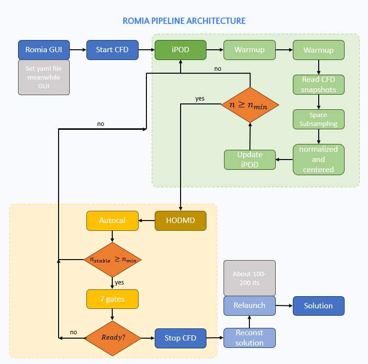
Figure 1. Conceptual architecture of the ROMIA pipeline. Snapshots from the running CFD simulation are compressed by iPOD, modelled by HODMD, and, once the trigger is satisfied, reconstructed and reinjected into the solver.
This conservative strategy is important for industrial CFD workflows. A failed prediction should not corrupt the final result: if the trigger is not satisfied, the original CFD simulation continues normally.
Parameter Tuning Guide
The quality of the acceleration depends on how well the reduced model represents the convergence transient. The parameters below are the most influential when preparing a ROMIA run.
Warmup iterations
The warmup phase lets the solver move away from the initial condition before ROMIA starts collecting snapshots. If warmup is too short, the basis captures the initial transient rather than the convergence path. If it is too long, ROMIA misses part of the useful convergence history and the potential acceleration decreases.
A practical starting point is to set warmup to the iteration at which the initial residual peak has subsided and the main flow structures are visible.
Snapshot interval and total number
The snapshot stride controls the temporal resolution of the reduced model. A stride of 1 or 2 is typical for RANS cases. If the stride is too large, HODMD may miss fast transient modes. If it is too small, disk and memory costs increase without improving the model.
The HODMD window needs enough snapshots to resolve the slowest decaying mode. As a rule of thumb, the window should contain at least a few cycles of the slowest transient feature observed in the coefficients.
iPOD energy threshold
The energy threshold η decides how many iPOD modes are retained. A value of 0.9999 keeps almost all captured energy and is a safe default. Reducing η decreases computational cost but may discard modes that carry relevant convergence information. For cases with a very low-dimensional transient, the number of retained modes will remain small even with a high threshold.
Spatial subsampling
Subsampling is recommended for meshes above a few million cells. It reduces the cost of building the iPOD basis and reconstructing the fields. The trade-off is an interpolation error, which is usually largest in high-gradient regions such as boundary layers or wakes.
If the validation errors are too high, try reducing the subsampling fraction or adding extra samples near walls and aerodynamic surfaces.
HODMD parameters
- Delay embedding
d: values between 10 and 40 work well for steady RANS convergence. Start with 20 and increase if the trigger reports poor spectral stability. - Window length: should be large enough to cover the slowest transient. Typical values range from 100 to 300 snapshots.
- Steady modes: usually 1 to 5. These correspond to the near-zero-frequency modes that dominate the asymptotic steady state. Too few modes smooth out the final state; too many may include spurious low-frequency transients.
When the trigger does not become READY
If the trigger remains inactive for a long time, consider the following actions:
- Increase
max_iterationsor the HODMD window to give the model more snapshots. - Reduce the snapshot stride to improve temporal resolution.
- Check that the selected fields are being written by OpenFOAM at the expected interval.
- Verify that the warmup is long enough for the solver to settle into a smooth convergence path.
- Relax overly strict trigger thresholds only if the physical validation remains conservative.
Case Study 1: Urban Flow
Case Description
The first practical case corresponds to an urban flow simulation based on a three-dimensional array of buildings. The objective is to demonstrate that ROMIA can accelerate a steady RANS simulation involving multiple bluff bodies, interacting wakes and recirculation zones.
Urban flow simulations are challenging because the flow is highly sensitive to wind direction, building arrangement and wake interaction. Even when the main flow structure is already formed, the final residual convergence can remain slow.
CFD Setup
| Parameter | Value |
|---|---|
| Geometry | 3D urban building array |
| Mesh cells | 2,062,043 |
| Domain | 3.0 m × 5.0 m × 1.0 m |
| Inlet velocity | U = 4.0 m/s (y-direction) |
| Reynolds number | Re ≈ 6.7 × 10⁴ |
| Solver | foamRun / incompressibleFluid |
| OpenFOAM version | 13 |
| Turbulence model | Standard k-epsilon (ABL modified) |
| Parallel execution | 8 processors |
The domain corresponds to a scaled wind-tunnel configuration. The inlet boundary uses a time-varying mapped velocity profile, while the buildings and ground are treated as no-slip walls. The k-epsilon coefficients include a modified sigmaEps = 1.11 following Hargreaves & Wright (2007) for atmospheric boundary layer flows.
ROMIA Configuration
For the urban case, ROMIA was configured in managed mode. The pipeline monitored the OpenFOAM simulation through filesystem polling and collected snapshots during the convergence transient.
| Parameter | Value |
|---|---|
| Mode | Managed |
| Solver | simpleFoam |
| Parallel | 8 processors |
| Fields | U, p |
| Subsampling | No subsampling |
| Warmup | 250 iterations |
| Write interval | 1 iteration |
| iPOD energy threshold | η = 0.9999 |
| iPOD max rank | 30 |
| HODMD delay embedding | d = 20 |
| HODMD autocalibration | Enabled, windows 150–300 snapshots |
| Trigger RMSE threshold | 0.15 |
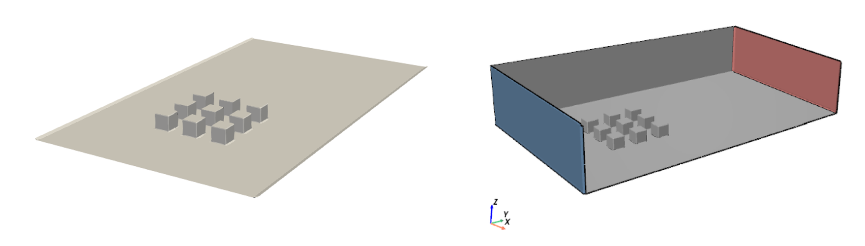
Figure 2. Urban flow case. Left: three-dimensional array of buildings. Right: boundary-condition patch view.
Why This Case Matters
This case is representative of CFD problems where the final solution is dominated by large-scale structures:
- Wakes behind buildings.
- Recirculation zones between obstacles.
- Strong local velocity gradients.
- Long RANS convergence tails.
- Sensitivity to the imposed incident wind direction.
The case therefore provides a useful validation step between simple aerodynamic benchmarks and more complex industrial geometries.
The limited number of retained modes — bounded by a maximum rank of 30 — indicates that the convergence transient evolves in a relatively low-dimensional subspace, despite the geometric complexity of the urban configuration.
Results
The urban case confirms that ROMIA can reproduce the dominant flow structures of the converged RANS solution. The predicted field captures the main wake topology, the inter-building recirculation regions and the global distribution of the dominant velocity component.
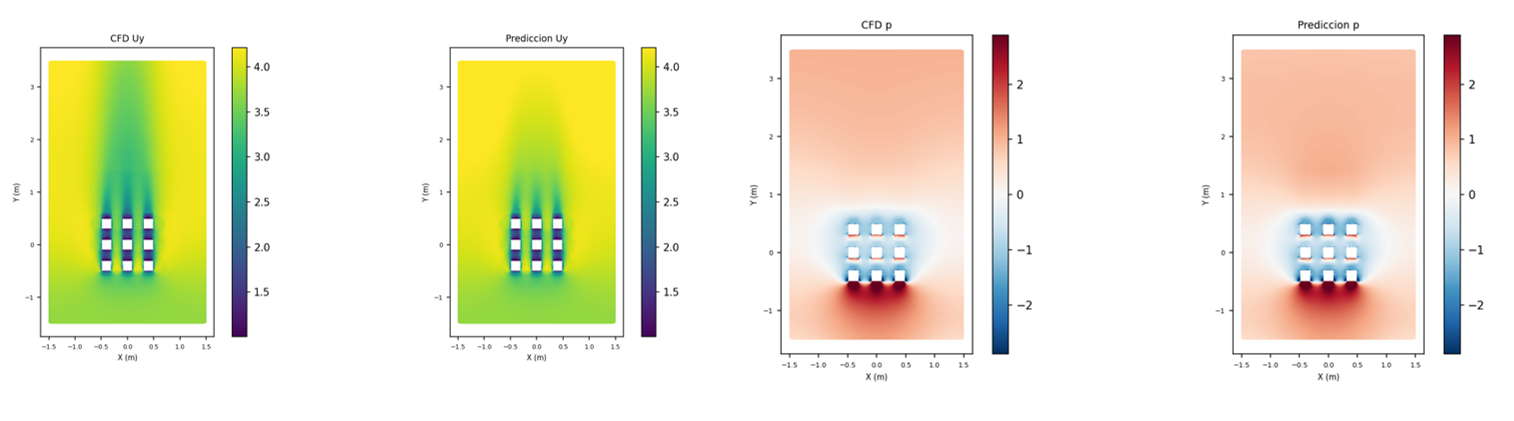
Figure 3. Comparison between the converged CFD reference and the ROMIA reconstructed field for the urban flow case.
The main conclusion from this case is that ROMIA is able to identify the asymptotic behaviour of an urban RANS simulation before full residual convergence is reached. This makes the method suitable for workflows where many wind directions or urban configurations must be evaluated.
Case Study 2: 3D Formula 1 Rear Wing
Case Description
The second practical case applies ROMIA to a three-dimensional Formula 1 rear wing. This case represents a more demanding industrial-scale CFD problem, with a large unstructured mesh, strong pressure gradients, wake development and separated turbulent structures.
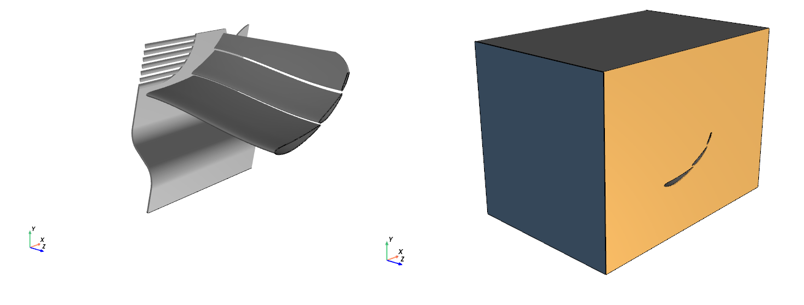
Figure 4. Three-dimensional Formula 1 rear wing geometry used as an industrial-scale validation case.
CFD Setup
| Parameter | Value |
|---|---|
| Geometry | 3D F1 rear wing |
| Mesh cells | 29,482,757 |
| Inlet velocity | U_inf = 73 m/s |
| Reynolds number | Re ≈ 3.5 × 10⁶ |
| Solver | simpleFoam |
| OpenFOAM version | OpenFOAM 2506 |
| Turbulence model | Standard k-epsilon |
| Parallel execution | 72 processors |
The case is representative of production aerodynamic simulations. It contains complex three-dimensional geometry, multiple aerodynamic elements, strong pressure gradients and a turbulent wake. These features make the final convergence stage expensive, especially when aerodynamic loads and pressure distributions must be stabilized accurately.
ROMIA Configuration
| Parameter | Value |
|---|---|
| Mode | Managed, filesystem polling |
| Spatial subsampling | 10% using cell_volume_sqrt |
| Warmup | 100 iterations |
| Snapshot range | Iterations 102–500 |
| Number of snapshots | 200 |
| Write interval | 2 iterations |
| iPOD energy threshold | η = 0.9999 |
| Retained modes | 80 |
| HODMD delay embedding | d = 20 |
| HODMD window | 180 snapshots |
| HODMD steady modes | 4 |
The larger number of retained modes compared with the urban case reflects the greater geometric and aerodynamic complexity of the rear wing configuration.
The spectral analysis of the iPOD basis confirms that the convergence transient is extremely low-dimensional. The first five modes retain 99.989% of the modal energy, and the basis stabilises at r = 80 modes after approximately 80 snapshots.
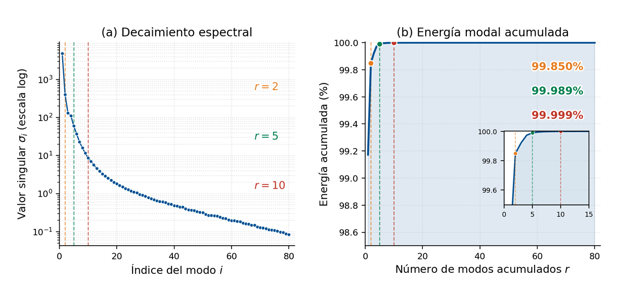
Figure 5. Spectral analysis of the iPOD basis for the F1 rear wing case. (a) Singular value decay. (b) Cumulative modal energy. Five modes retain 99.989% of the energy.
Pressure Field Prediction
The pressure field is one of the most relevant outputs in external aerodynamics, since it is directly related to the aerodynamic forces generated by the wing. ROMIA reconstructs the main pressure distribution over the rear wing while reducing the wall-clock time required to reach a validated solution.
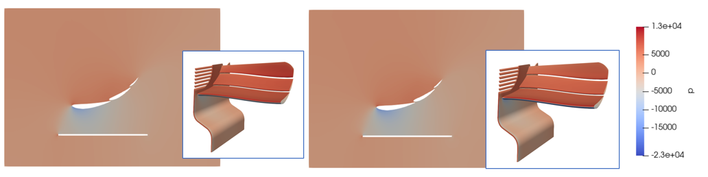
Figure 6. Pressure field comparison. Left: ROMIA prediction. Right: converged pure CFD reference.
Velocity Field Prediction
The velocity magnitude comparison shows that the reconstructed field preserves the global wake structure and the main acceleration regions around the aerodynamic elements.
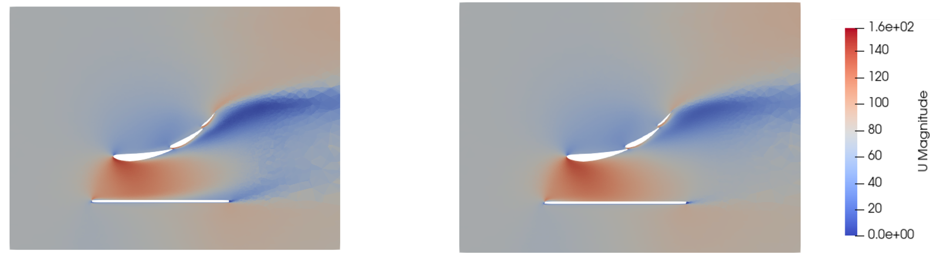
Figure 7. Velocity magnitude comparison. Left: ROMIA prediction. Right: converged pure CFD reference.
Validation Against Reference CFD
The ROMIA prediction at iteration 10200 is compared against a pure CFD reference run on the same mesh. The local error maps below show the pointwise discrepancy normalised by the range of the reference field. The largest deviations occur in the far wake and in regions of high gradient, where the modal reconstruction smooths small-scale structures that the solver develops in later iterations.
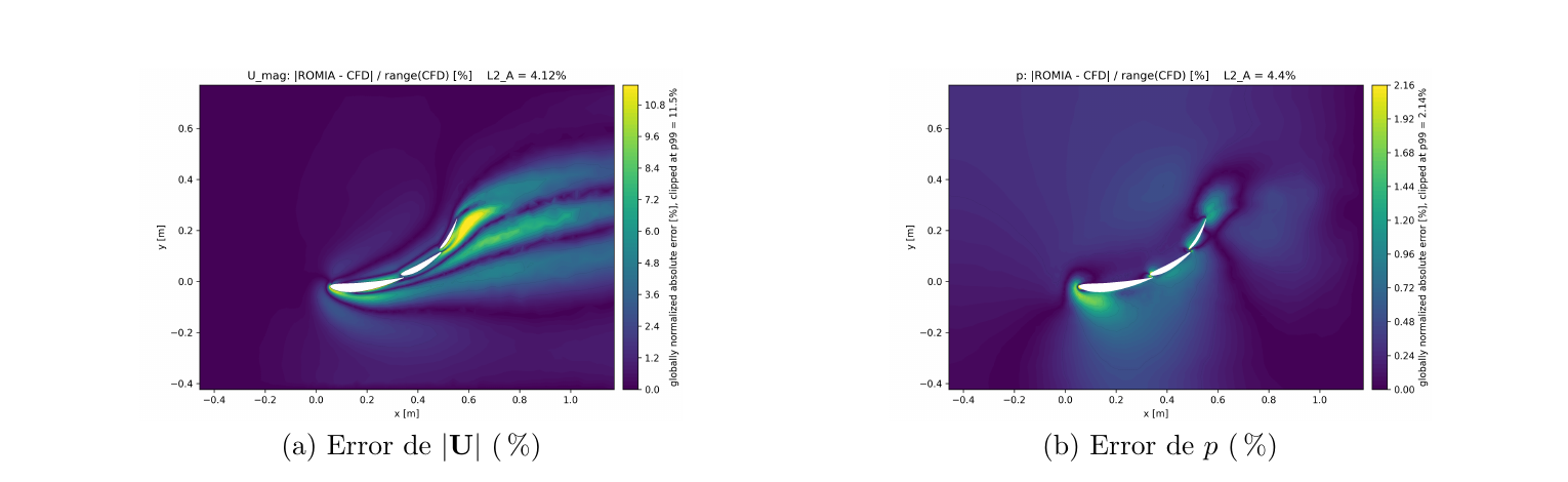
Figure 8. Local error maps of ROMIA against the pure CFD reference on the plane z = 0.5 m. (a) Velocity magnitude |U|. (b) Pressure p. Errors are normalised by the range of the reference field.
The area-weighted L₂ errors on the analysed cut plane are:
| Field | L₂,A |
|---|---|
| Velocity magnitude |U| | 4.12 % |
| Pressure p | 4.40 % |
These values indicate that the restarted field converges to a solution compatible with the reference CFD for the aerodynamic quantities of interest.
Computational Acceleration
The full CFD simulation required 15 h 54 min, while the ROMIA-accelerated workflow reached a validated solution in 6 h 32 min.
| Workflow | Wall-clock time |
|---|---|
| Pure CFD | 15 h 54 min |
| ROMIA-accelerated CFD | 6 h 32 min |
| Speed-up | ≈ 2.5× |
| Time reduction | ≈ 60% |
This result demonstrates that ROMIA can provide significant acceleration on large-scale industrial CFD cases while preserving the global flow structure and the relevant aerodynamic behaviour.
Practical Recommendations
ROMIA is designed to support practical CFD workflows, but it should be used with the same verification mindset as any acceleration or numerical modelling tool.
Post-restart validation checklist
After ROMIA reinjects the reconstructed fields, verify the following before accepting the result:
- Residual behaviour. The residuals should decay smoothly after the restart. A sudden growth, plateau or oscillation is a sign that the prediction was premature or that the reduced basis was insufficient.
- Flow topology. Compare the main flow structures — wakes, recirculation bubbles, separation lines — against the pre-restart field and against engineering expectations.
- Field bounds. Check that pressure, velocity magnitude, turbulence variables and
chi = epsilon/kremain within physical ranges. Negative turbulence quantities or extreme local spikes indicate a problem. - Convergence history. Continue the simulation until the residuals reach the same convergence criterion used for the reference CFD run.
Case-specific advice
- External aerodynamics: pay special attention to pressure distribution along aerodynamic surfaces and to force coefficients. The boundary layer and trailing-edge pressure are sensitive indicators.
- Urban flows: focus on wake topology, inter-building recirculation zones and velocity profiles at pedestrian or sensor locations.
- Turbulent restarts: when using the
k-epsilonpolicy, inspectk,epsilonandnutfor non-physical values in the first iterations after reinjection.
Troubleshooting and FAQ
The trigger never becomes READY
- Make sure the OpenFOAM simulation is writing the selected fields at the configured interval.
- Increase the warmup or the maximum number of iterations. The convergence transient may be slower than expected.
- Reduce the snapshot stride to give HODMD more temporal resolution.
- Check that the iPOD basis is capturing enough energy. If too few modes are retained, increase
ηor reducemax_rankconstraints.
The simulation diverges after restart
- Verify that the warmup was long enough. A prediction based on the initial transient often leads to an unstable restart.
- Reduce the HODMD steady-mode count if the reconstructed state contains spurious low-frequency oscillations.
- Check turbulence variables. If
k-epsilonis not used, ROMIA may not apply a model-aware policy for turbulence. - Consider reducing spatial subsampling or adding boundary samples if high-gradient regions are poorly reconstructed.
The errors against reference CFD are too high
- Increase the number of retained iPOD modes or raise
η. - Lengthen the HODMD window so that slow convergence modes are better resolved.
- Reduce subsampling fraction or use a strategy that preserves wall and wake regions.
- Compare the error distribution. Localised errors in the far wake are expected; errors on aerodynamic surfaces or in the main flow path should be small.
What happens if I use k-omega SST or Spalart-Allmaras?
ROMIA detects these turbulence models, but the model-aware restart policy is currently implemented only for standard k-epsilon. If another turbulence model is selected, ROMIA will still reconstruct the mean fields (velocity and pressure) and the turbulence variables, but the algebraic consistency guarantees of the chi = epsilon/k transformation do not apply. In this situation, post-restart validation of k, omega or nut becomes especially important.
Can ROMIA be used for unsteady flows?
No. ROMIA is designed for steady or quasi-steady RANS simulations. Phenomena such as vortex shedding, travelling instabilities or long transients are outside the current scope.
Does ROMIA modify my OpenFOAM case?
No. ROMIA reads the fields written by the solver and writes a new restart directory. The original system, constant and 0 directories are not modified.
Current Limitations
ROMIA does not replace the CFD solver and should not be interpreted as a black-box converged-solution generator. Its purpose is to generate a better restart condition than the current intermediate CFD state.
The final solution must always be validated by continuing the original CFD simulation. The quality of the acceleration depends on the representativeness of the collected snapshots, the stability of the reduced-order model and the physical consistency of the reconstructed variables.
Current limitations include:
- Turbulence model support. The model-aware turbulent restart policy is fully supported only for the standard
k-epsilonmodel.k-omega SSTandSpalart-Allmarasare detected but do not yet have a dedicated ROM policy. When these models are used, ROMIA reconstructs the fields without thechitransformation and relies on the standard post-restart validation. - Steady-state scope. ROMIA is designed for steady or quasi-steady RANS simulations. It has not been validated for long transients or inherently unsteady phenomena such as vortex shedding or convective instabilities.
- Spatial growth of turbulent structures. HODMD modes have a fixed spatial structure with purely temporal evolution, so ROMIA cannot represent structures that grow spatially (e.g., wake lengthening downstream). Nonlinear or extended-dimension methods would be required.
- Subsampling interpolation error. Reconstruction from spatial subsamples introduces interpolation error in high-gradient regions, which may require additional local refinement.
Future Work
Several development lines are currently being considered to extend ROMIA:
- Extended turbulence-model support, in particular a model-aware policy for
k-omega SSTvia transformation to the model’s characteristic variables. - Nonlinear compression, using deep autoencoders as an alternative spatial compression backend for cases where linear POD becomes restrictive.
- MPI parallelisation of iPOD, to reduce overhead on meshes with billions of cells.
- Broader industrial validation, through systematic testing on wind turbines, full vehicles and additional urban configurations.
Summary
ROMIA provides a practical, non-intrusive framework for accelerating steady-state CFD simulations. By combining online field monitoring, incremental modal compression, HODMD-based temporal prediction and a conservative multilayer trigger, ROMIA can generate physically consistent restart fields that reduce the cost of the final convergence stage.
The two practical cases presented here illustrate the range of applicability of the method:
- The urban flow case shows that ROMIA can capture the dominant wake and recirculation structures of a multi-building RANS simulation with up to 30 retained modes.
- The 3D F1 rear wing case demonstrates industrial-scale acceleration on a 29.5-million-cell mesh, reducing wall-clock time from 15 h 54 min to 6 h 32 min while preserving the main pressure and velocity structures.
ROMIA is therefore not only a reduced-order modelling method, but also a practical CFD workflow tool: it allows the user to accelerate simulations while keeping the original solver responsible for final validation.
Further Reading
- Theoretical background on HODMD: Le Clainche & Vega, SIAM Journal on Applied Dynamical Systems, 2017
- Modal selection criterion: Kou, Le Clainche & Zhang, Physics of Fluids, 2018
- ModelFLOWs App: https://modelflows.github.io/modelflowsapp/