Overview
This tutorial explains how to reconstruct full 3D urban flow and pollutant fields from sparse sensor information. The workflow is based on low-cost reduced-order modelling methods, where only a reduced set of points is used to recover the original high-dimensional CFD field.
The tutorial includes three reconstruction methods:
- lcSVD
- lcHOSVD
- lcHODMD
lcSVD and lcHOSVD are mainly used for spatial 3D reconstruction. lcHODMD is used for dynamic reconstruction, where the objective is to recover time-resolved flow structures from reduced information.
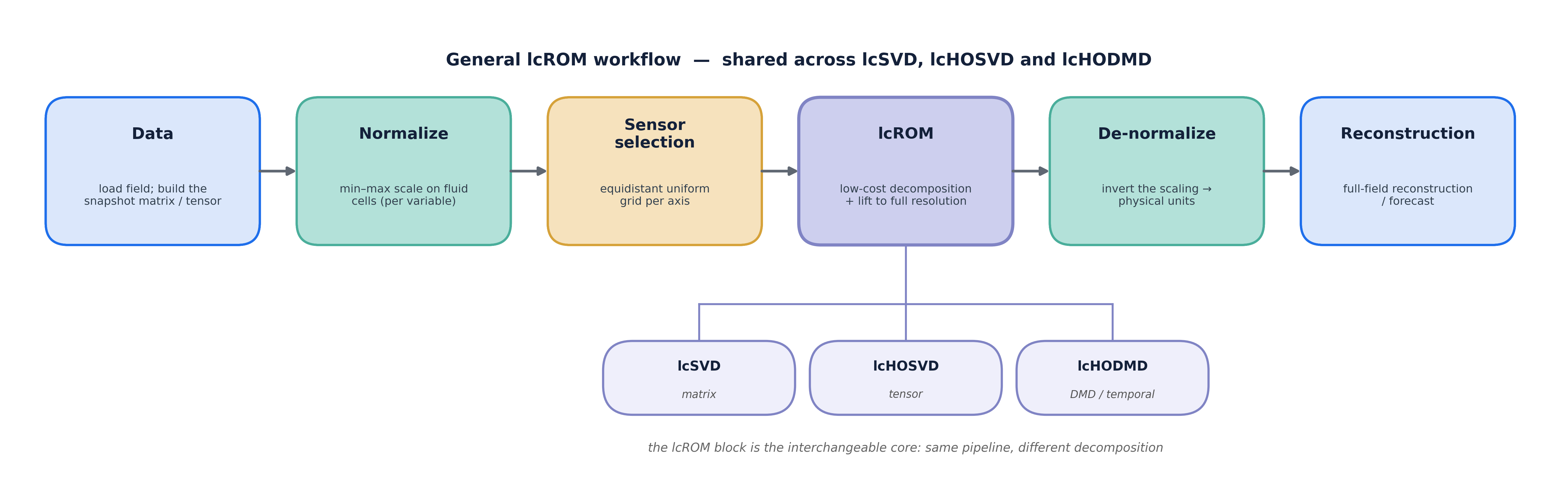
General low-cost reduced-order modelling workflow for reconstructing high-dimensional flow databases from sparse sensor information.
Learning Objectives
- Load and prepare 3D urban CFD data.
- Select sparse sensor locations from the full computational domain.
- Choose modes for both lcSVD and lcHOSVD.
- Reconstruct full 3D fields using lcSVD.
- Reconstruct full 3D fields using lcHOSVD.
- Apply lcHODMD for dynamic reconstruction.
- Select important HODMD parameters such as delay dimension
dand toleranceepsilon. - Compare reconstructed fields with the ground truth.
- Evaluate reconstruction error, compression, and computational time.
- Visualize reconstructed urban flow and pollutant fields.
Requirements
- Python: 3.9.18
- NumPy: 1.26.4
- SciPy: 1.13.1
- Matplotlib: 3.9.0
- scikit-learn: 1.5.0
Input Data
- Urban CFD dataset
- Sparse sensor locations
- Ground-truth 3D fields
- Velocity components
- Pressure field
- Pollutant concentration fields
- Time-resolved snapshots
Step-by-Step Tutorial
Step 1. Load the urban CFD field
Load the CFD field or processed tensor containing the physical variables of interest.
Typical variables include:
- velocity component
u; - velocity component
v; - velocity component
w; - pressure;
- turbulent kinetic energy;
- pollutant concentration fields such as CO, NOx, PM10, or PM2.5.
The data should be arranged so that the 3D structure of the domain is preserved.
Step 2. Select the reconstruction variable
Choose the variable to reconstruct.
Each variable can be reconstructed independently or together at once. For example, one can first reconstruct u, then repeat the same workflow for v, w, pressure, or pollutant concentration.
Step 3. Define the full-order reference field
Prepare the ground-truth field that will be used as the reference solution.
This field is required for:
- computing reconstruction error;
- comparing original and reconstructed snapshots;
- checking spatial structures;
- validating whether the reduced method preserves the main physical behaviour.
Step 4. Select sparse sensor locations
Select a reduced number of points from the full computational domain.
The sensor grid should be sufficiently representative of the flow field. A sparse grid reduces the computational cost, but too few sensors may miss important spatial structures.
The selected sensors are used to build the reduced dataset for lcSVD, lcHOSVD, and lcHODMD.
Step 5. Apply lcSVD reconstruction
Apply low-cost SVD to reconstruct the full 3D field from sparse sensor information.
In lcSVD, the 3D field is reshaped into a matrix. The sparse sensor matrix is then decomposed, and a selected number of modes is retained.
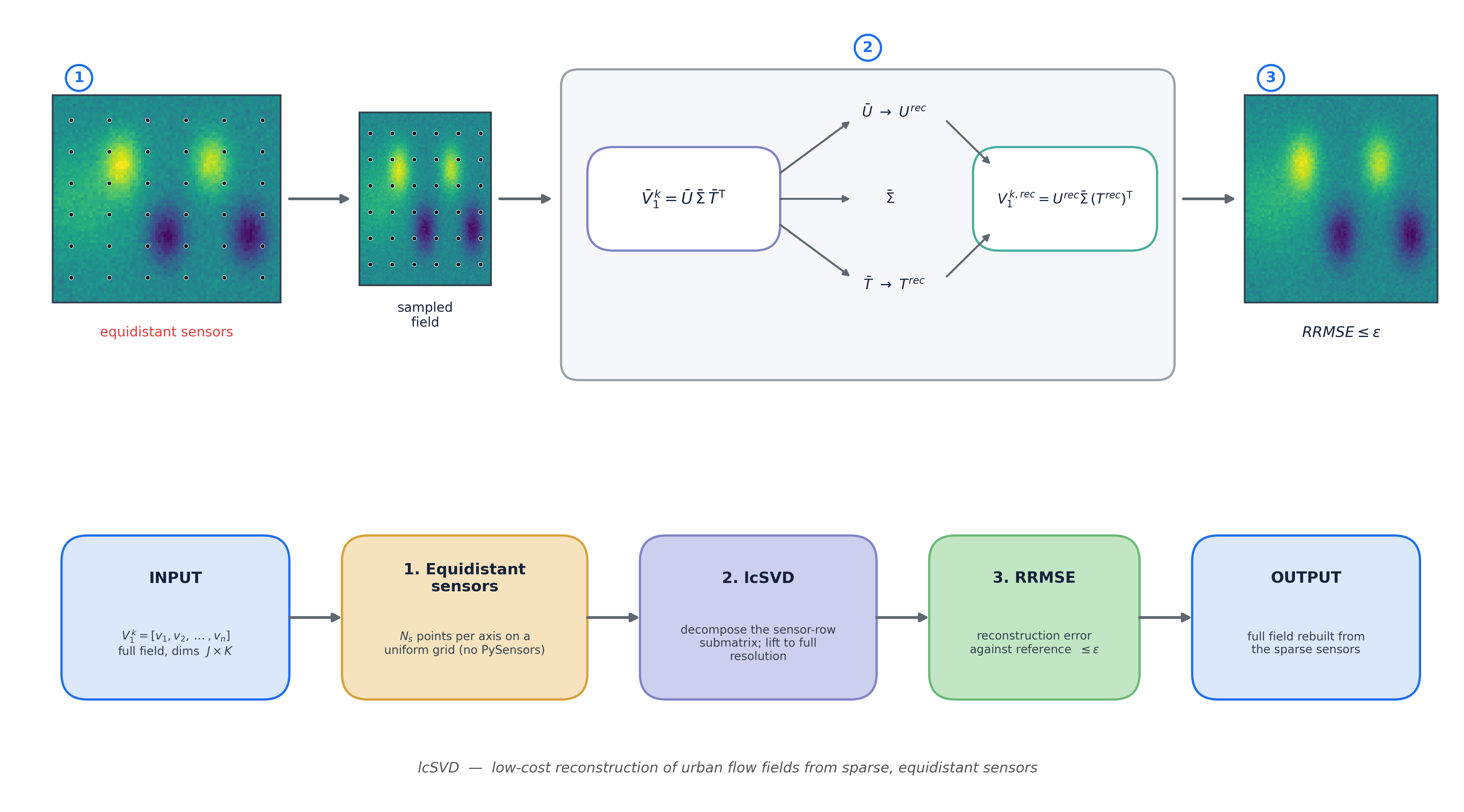
Low-cost SVD workflow for reconstructing the full field from a reduced matrix built using sparse sensor locations.
The main steps are:
- reshape the 3D field into matrix form;
- extract the sensor rows or sensor points;
- apply SVD to the reduced matrix;
- select the number of retained modes;
- reconstruct the full field;
- compare the result with the ground truth.
The main outputs are:
- lcSVD reconstructed field;
- retained SVD modes;
- singular values;
- reconstruction error;
- computational time;
- compression ratio.
Step 6. Apply lcHOSVD reconstruction
Apply low-cost HOSVD to reconstruct the field while preserving the tensor structure of the 3D domain.
Unlike lcSVD, lcHOSVD keeps the spatial directions separated. This is useful when the flow has directional structures in the x, y, and z directions.
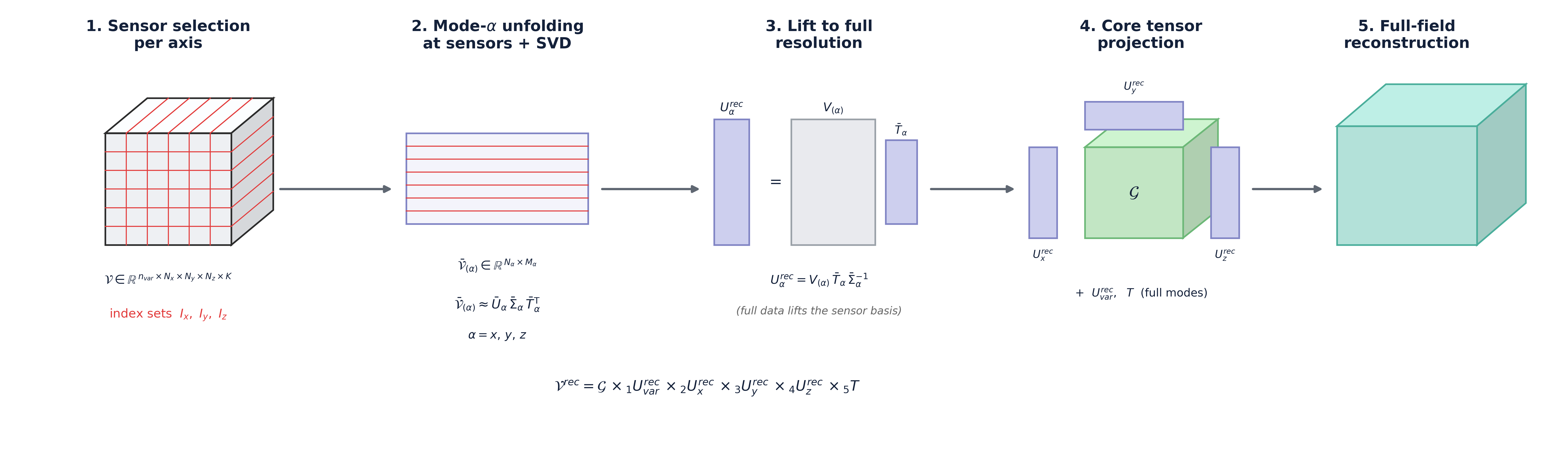
Low-cost HOSVD workflow for tensor-based reconstruction, where spatial directions are treated separately and coupled through a compact core tensor.
The main steps are:
- arrange the field as a tensor;
- select the sparse sensor tensor;
- choose the retained modes in each spatial direction;
- apply HOSVD to the reduced tensor;
- reconstruct the full tensor field;
- compare the reconstructed field with the ground truth.
The main outputs are:
- lcHOSVD reconstructed field;
- spatial modes in each direction;
- compact core tensor;
- reconstruction error;
- computational time;
- comparison with lcSVD.
Step 7. Apply lcHODMD reconstruction
Apply low-cost HODMD to reconstruct the time-resolved flow field from reduced information.
lcHODMD is useful when the dataset contains temporal evolution. Instead of reconstructing only one static field, the method reconstructs a sequence of snapshots by extracting dynamic modes and temporal behaviour.
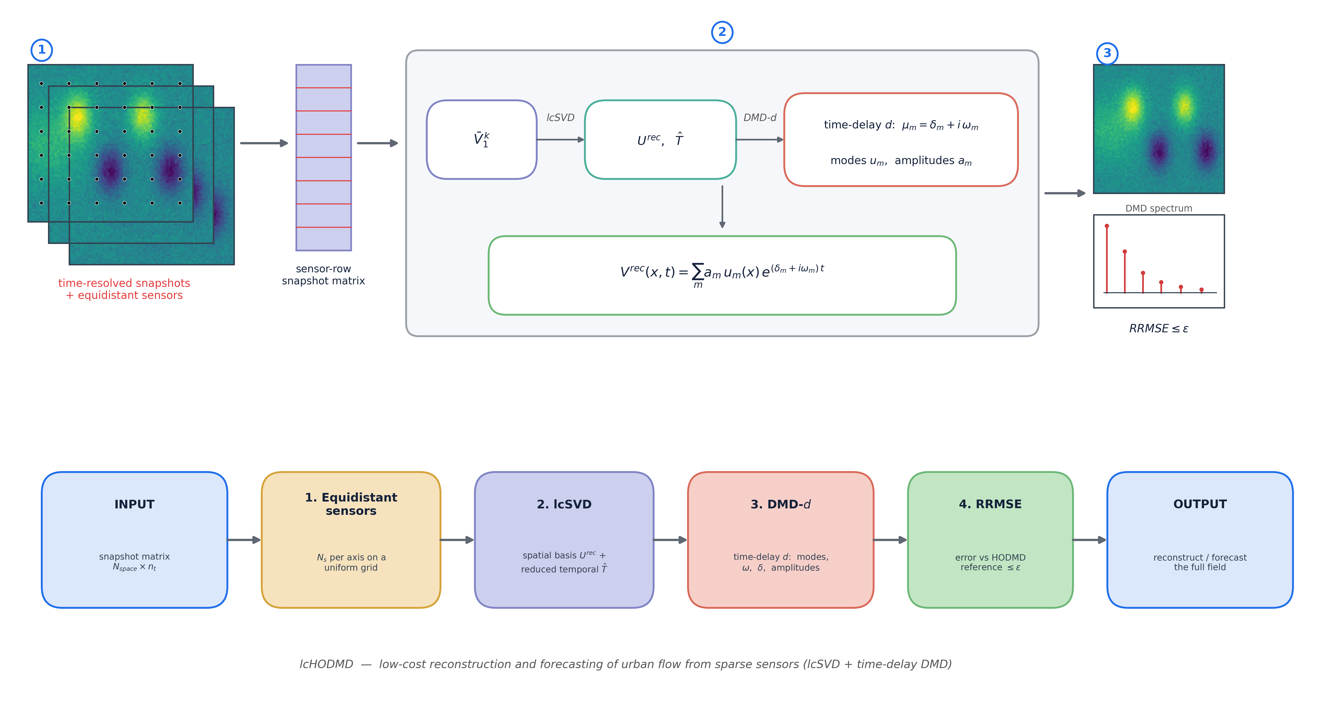
Low-cost HODMD workflow for recovering time-resolved flow structures from a reduced dynamic representation.
The important HODMD parameters are:
d: delay dimension or number of delayed snapshots;epsilon: tolerance used to truncate small singular values or weak modes;svd_rank: number of retained modes or automatic rank selection;dt: time step between snapshots;- number of snapshots used for reconstruction;
- number of snapshots used for validation.
Step 8. Select the HODMD delay dimension d
The delay dimension d controls how many delayed snapshots are used to build the higher-order representation.
A small value of d may not capture enough temporal memory. A very large value may increase computational cost and may introduce unnecessary modes.
Step 9. Select the HODMD tolerance epsilon
The tolerance epsilon controls the truncation of weak singular values or modes.
A larger tolerance removes more modes and gives a more compact model. A smaller tolerance retains more information but may also keep noise or weak dynamics.
Step 10. Build the delayed snapshot matrix
Construct the delayed snapshot representation using the selected value of d.
This step allows HODMD to capture richer temporal dynamics than standard DMD. The delayed structure is especially useful for flow fields where the dominant dynamics are not fully described by two consecutive snapshots.
Step 11. Extract dynamic modes
Apply HODMD to the reduced delayed dataset.
The method extracts:
- dynamic modes;
- modal amplitudes;
- frequencies;
- growth rates;
- temporal coefficients.
These quantities describe how the flow evolves in time.
Step 12. Reconstruct the time-resolved field
Use the retained dynamic modes and temporal coefficients to reconstruct the flow snapshots.
The reconstructed snapshots are then compared with the reference CFD data.
Expected Outputs
- lcSVD reconstructed 3D fields.
- lcHOSVD reconstructed 3D fields.
- lcHODMD reconstructed time-resolved snapshots.
- Dynamic modes.
- Modal amplitudes.
- Frequencies and growth rates.
- Reconstruction error tables.
- Ground-truth versus reconstructed visualizations.
- Computational time and compression comparison.
Related Links
- Notebook: coming soon
- Video: coming soon
- Dataset: coming soon
- Repository: coming soon
- Research page: From Sensors to 3D Reconstruction
- Application page: Urban Flows
Contributors
- Arindam Sengupta
- Soledad Le Clainche