Overview
This tutorial explains how to calibrate low-cost air-quality sensor measurements using temporal deep learning.
Low-cost sensors are useful for dense urban monitoring, but their raw measurements can be affected by drift, environmental cross-sensitivity, and changing field conditions. The calibration workflow uses reference-grade observations and meteorological variables to correct the low-cost sensor output.
The workflow focuses on LSTM-based calibration of pollutant measurements such as:
- PM2.5
- PM10
- NO2
Learning Objectives
- Load low-cost sensor and reference data.
- Align sensor measurements with reference observations.
- Prepare meteorological and pollutant-specific variables.
- Create lagged and temporal features.
- Generate rolling-window sequences.
- Train an LSTM calibration model.
- Evaluate calibrated outputs using R2, MAE, and RMSE.
- Compare raw sensor data, calibrated predictions, and reference measurements.
- Assess model performance on unseen data.
Requirements
- Python: 3.9.18
- NumPy: 1.26.4
- Pandas: 2.2.2
- Matplotlib: 3.9.0
- scikit-learn: 1.5.0
- TensorFlow / Keras : 2.10.0
Input Data
- Low-cost sensor measurements
- Reference air-quality measurements
- Meteorological variables
- Pollutant-specific sensor variables
- Baseline-corrected sensor data
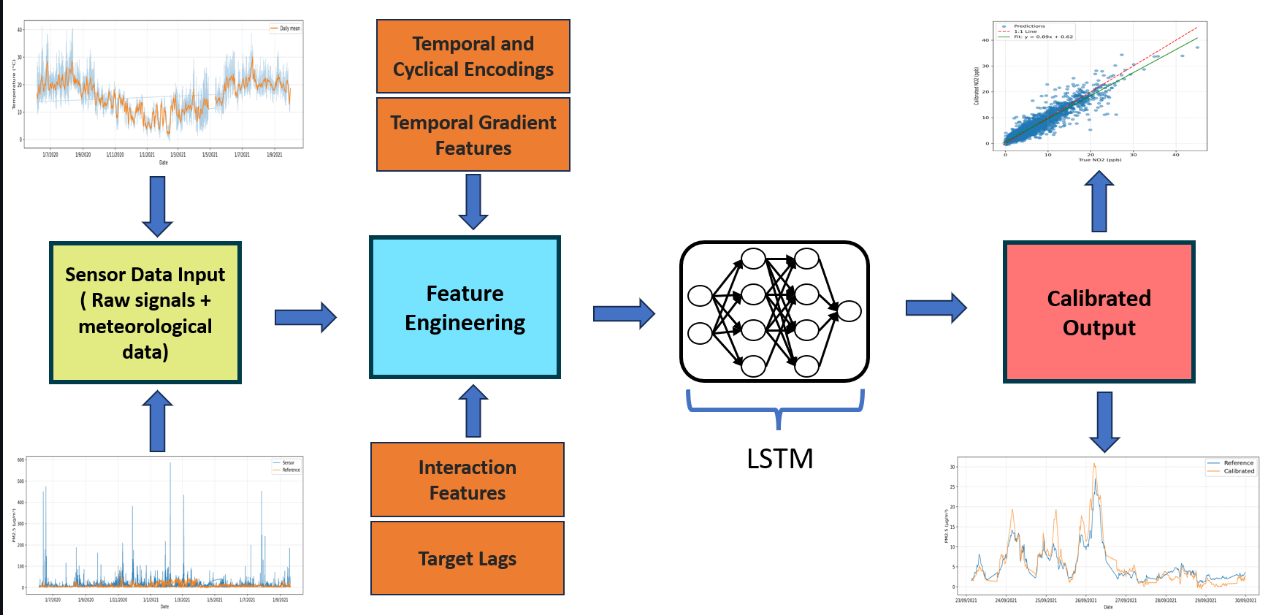
Methodology for the temporal calibration of low-cost air-quality sensors.
Step-by-Step Tutorial
Step 1. Load low-cost sensor data
Load the low-cost sensor measurements for the pollutant of interest.
The sensor data may include:
- raw pollutant concentration;
- sensor voltages;
- optical particle counter variables;
- sample flow rate;
- sample time of flight;
- temperature;
- relative humidity.
Step 2. Load reference measurements
Load the co-located reference-grade observations.
These reference values are used as the target data during supervised calibration.
Step 3. Align data by timestamp
Synchronize the low-cost sensor data and the reference measurements.
Each sensor measurement should correspond to the correct reference value and meteorological condition.
Step 4. Clean the dataset
Remove or correct:
- missing values;
- invalid records;
- duplicated timestamps;
- physically unrealistic values;
- incomplete time intervals.
This step is important because calibration quality depends strongly on the quality of the input data.
Step 5. Select pollutant-specific input variables
Choose the input variables depending on the pollutant.
For particulate matter, useful variables may include:
- sensed particle mass;
- sample flow rate;
- sample time of flight;
- temperature;
- relative humidity.
For NO2, useful variables may include:
- sensed concentration;
- working electrode voltage;
- auxiliary electrode voltage;
- temperature;
- relative humidity.
Step 6. Create engineered features
Create additional features to help the model capture temporal behaviour and environmental effects.
The engineered features may include:
- lagged pollutant values;
- lagged meteorological variables;
- short-term percentage changes;
- hour of day;
- day of week;
- rush-hour indicators;
- harmonic time encodings;
- interaction terms between sensor and environmental variables.
Step 7. Normalize the data
Scale the input features before training the neural network.
Normalization improves numerical stability and helps the model learn from variables with different units and magnitudes.
The same scaling parameters should be used later for validation, testing, and unseen data.
Step 8. Generate rolling-window sequences
Convert the calibrated dataset into a sequence-to-one learning problem.
The model receives a fixed window of previous observations and predicts the calibrated pollutant concentration at the next time step.
This allows the LSTM model to learn:
- temporal persistence;
- delayed environmental effects;
- sensor memory;
- short-term pollutant dynamics.
Step 9. Split the data
Split the sequence dataset into:
- training set;
- validation set;
- test set.
The split should preserve temporal order to avoid information leakage from the future into the past.
Step 10. Define the LSTM calibration model
Build the LSTM model for temporal calibration.
A typical model includes:
- input sequence layer;
- LSTM layer;
- dense layer;
- dropout or regularization;
- final linear output layer.
The model predicts the calibrated pollutant concentration.
Step 11. Train the model
Train the model using the training set and monitor performance on the validation set.
Early stopping can be used to avoid overfitting.
Step 12. Evaluate the calibrated output
Evaluate the trained model using the test set.
Common metrics include:
- R2;
- MAE;
- RMSE.
The calibrated output should be compared with the reference measurement and the raw low-cost sensor signal.
Expected Outputs
- Cleaned calibration dataset.
- Engineered feature table.
- Rolling-window sequences.
- Trained LSTM calibration model.
- Calibrated pollutant concentration.
- Validation and test metrics.
- Unseen-data evaluation.
- Scatter plots against reference observations.
- Time-series comparison.
- Raw sensor versus calibrated output plots.
Related Links
- Notebook:LCS calibration
- Video: coming soon
- Dataset: OxAria low-cost air-quality sensor dataset
- Repository: coming soon
- Research page: Temporal Deep Learning Calibration of Low-Cost Air Quality Sensors
- Application page: Urban Flows
Publications
Contributors
- Arindam Sengupta
- Tony Bush
- Ben Marner
- Jose Miguel Pérez
- Soledad Le Clainche