Overview
This tutorial explains how to forecast the temporal evolution of urban flow fields using multidimensional higher-order dynamic mode decomposition.
The objective is to predict future flow states without rerunning the full CFD simulation. The method uses time-resolved data, extracts dominant temporal dynamics, and forecasts future snapshots from the reduced modal representation.
The workflow includes:
- data preparation;
- normalization;
- sequence generation;
- selection of mdHODMD parameters;
- selection of delay dimension
d; - selection of tolerance
epsilon; - forecasting future snapshots;
- autoregressive prediction;
- reconstruction of the predicted physical fields;
- comparison with the ground truth.
Learning Objectives
- Load time-resolved urban flow data.
- Prepare multidimensional data for mdHODMD.
- Normalize physical variables before decomposition.
- Generate temporal sequences for forecasting.
- Select mdHODMD parameters such as
dandepsilon. - Apply mdHODMD for modal decomposition.
- Forecast future snapshots.
- Apply autoregressive prediction.
- Reconstruct predicted fields in physical space.
- Compare predicted fields with reference CFD snapshots.
Requirements
- Python: 3.9.18
- NumPy: 1.26.4
- Pandas: 2.2.2
- Matplotlib: 3.9.0
- scikit-learn: 1.5.0
- TensorFlow / Keras : 2.10.0
Input Data
- Time-resolved urban CFD snapshots
- Velocity components
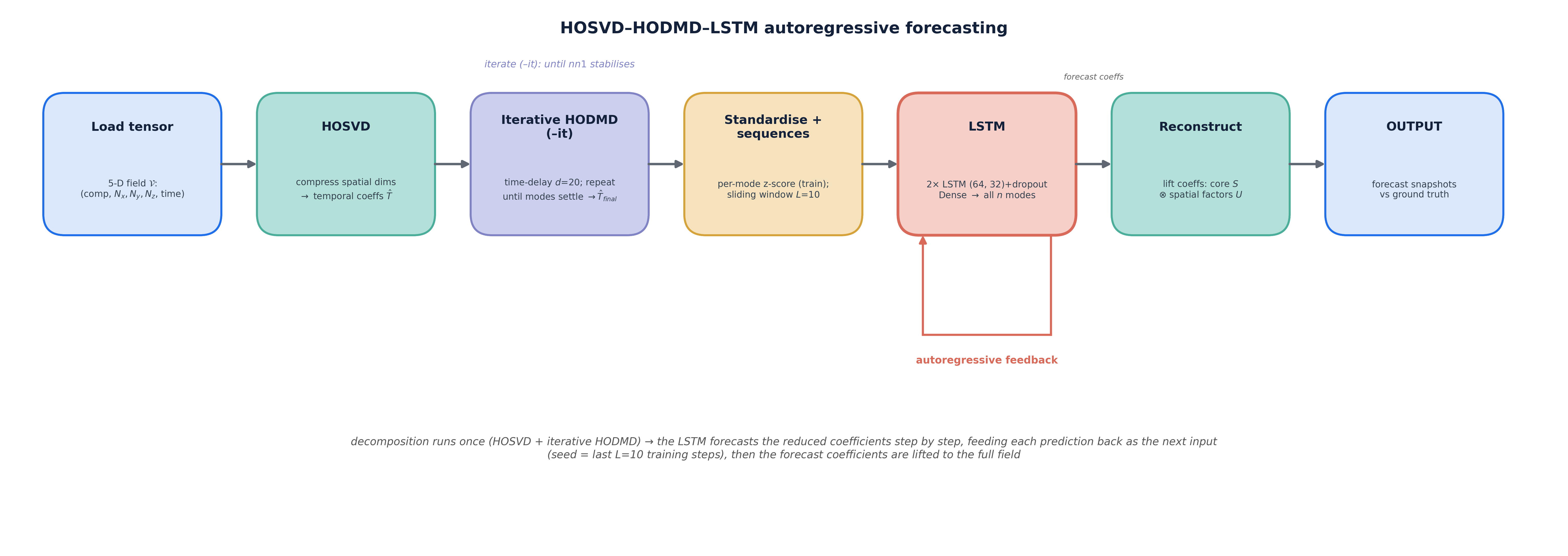
Iterative mdHODMD methodology for forecasting time-resolved urban flow and pollutant fields.
Step-by-Step Tutorial
Step 1. Load the time-resolved dataset
Load the sequence of CFD snapshots used for forecasting.
The dataset should contain the temporal evolution of the selected variable or group of variables.
Typical examples include:
- velocity components;
- pressure;
- turbulent quantities;
- pollutant concentration fields.
Step 2. Select the forecasting variable
Choose the field to forecast.
The workflow can be applied to one variable at a time or to multiple variables depending on the structure of the input tensor.
Step 3. Split the data into training and prediction windows
Separate the available snapshots into:
- snapshots used to learn the temporal dynamics;
- snapshots used as ground truth for forecast validation.
The training window is used by mdHODMD to identify modal dynamics. The prediction window is used to evaluate how well the method forecasts future states.
Step 4. Normalize the data
Normalize the selected variable before applying mdHODMD.
Normalization is important because different physical variables may have different magnitudes. It also improves numerical stability and avoids the decomposition being dominated by high-amplitude variables.
After prediction, the data should be transformed back to the original physical scale.
Step 5. Prepare the multidimensional structure
Arrange the dataset in multidimensional form.
Instead of flattening everything immediately, mdHODMD keeps the multidimensional structure of the problem as much as possible. This is useful for urban flow fields, where the spatial directions and physical variables contain meaningful structure.
Step 6. Generate temporal sequences
Create temporal sequences from the time-resolved snapshots.
The sequence length defines how many past snapshots are used to represent the current temporal state. This step prepares the data for higher-order temporal analysis and for later autoregressive prediction.
The sequence generation should define:
- input time window;
- number of past snapshots;
- forecast horizon;
- time step between snapshots;
- number of future snapshots to predict.
Step 7. Choose the delay dimension d
Select the HODMD delay dimension d.
The parameter d controls the number of delayed snapshots used in the higher-order representation. It determines how much temporal memory the model uses.
A small value of d may miss important temporal behaviour. A very large value of d may increase cost and may introduce weak or noisy modes.
The value of d should be selected by checking:
- prediction error;
- reconstructed training accuracy;
- number of modes retained;
- stability of the modes;
- quality of predicted flow structures.
Step 8. Choose the tolerance epsilon
Select the truncation tolerance epsilon.
This parameter controls which modes are retained and which are discarded. A larger tolerance gives a more compact model. A smaller tolerance keeps more modes but can retain noise.
The selected value should provide a balance between:
- prediction accuracy;
- numerical stability;
- number of modes;
- computational cost.
Step 9. Apply mdHODMD
Apply multidimensional HODMD to the training data.
The method extracts:
- spatial-temporal modes;
- modal amplitudes;
- temporal frequencies;
- growth or decay rates;
- reduced temporal representation.
These quantities describe the temporal behaviour learned from the training snapshots.
Step 10. Forecast future snapshots
Use the mdHODMD temporal dynamics to forecast snapshots beyond the training window.
The predicted snapshots represent the future evolution of the urban flow or pollutant field.
Step 11. Apply autoregressive prediction
For longer forecasts, use autoregressive prediction.
In autoregressive prediction, the predicted snapshot is fed back into the prediction process to estimate the next snapshot. This allows the model to move forward step by step beyond the initial forecast horizon.
The autoregressive loop follows this idea:
- use the available sequence to predict the next snapshot;
- append the predicted snapshot to the sequence;
- remove the oldest snapshot from the sequence;
- predict the next future snapshot;
- repeat until the required forecast length is reached.
This is useful when the objective is to generate a continuous future time series.
Step 12. Reconstruct the predicted physical fields
Convert the forecasted reduced representation back into the full physical field.
If normalization was applied earlier, apply the inverse transformation to recover the original physical scale.
Step 13. Compare prediction with ground truth
Compare the predicted snapshots with the available reference CFD data.
The comparison may include:
- predicted versus ground-truth fields;
- temporal error evolution;
- RRMSE;
- spatial error maps;
- pollutant concentration comparison;
- preservation of dominant flow structures.
Expected Outputs
- mdHODMD modes.
- Modal amplitudes.
- Temporal frequencies.
- Growth or decay rates.
- Reconstructed training snapshots.
- Forecasted future snapshots.
- Autoregressive prediction sequence.
- Prediction error values.
- Ground-truth versus forecasted field plots.
- Temporal error curves.
- Reconstructed physical fields.
Related Links
- Notebook: coming soon
- Video: coming soon
- Dataset: coming soon
- Repository: coming soon
- Application page: Urban Flows
Contributors
- Arindam Sengupta
- Soledad Le Clainche