Temporal Deep Learning Calibration of Low-Cost Air Quality Sensors
Low-cost air-quality sensors provide a practical way to increase the spatial density of urban monitoring networks. They are cheaper and easier to deploy than regulatory-grade instruments, making them useful for local pollution mapping, exposure assessment, and real-time environmental monitoring.
However, low-cost sensors are affected by sensor drift, environmental cross-sensitivity, device-to-device variability, and changing field conditions. Their raw measurements can therefore deviate strongly from reference-grade instruments, especially under variations in temperature, humidity, traffic activity, and seasonal conditions.
In this project, we develop a temporal deep learning framework for calibrating low-cost air-quality sensors. The method is designed for PM2.5, PM10, and NO2, and is trained using co-located reference data from the OxAria sensor network in Oxford, UK.
Unlike static calibration models such as Random Forest, which treat each observation independently, the proposed framework uses a Long Short-Term Memory network to learn temporal dependencies, delayed environmental effects, and evolving sensor behaviour.
The work is organized around four main steps:
-
Baseline-corrected sensor data preparation
Low-cost sensor measurements are combined with co-located reference observations and meteorological variables. -
Feature engineering and preprocessing
Lagged variables, temporal features, harmonic encodings, and interaction terms are constructed. -
LSTM-based temporal calibration
Fixed-length rolling windows are used to train a sequence-based calibration model. -
Validation and regulatory assessment
Calibrated outputs are evaluated using standard regression metrics and the Equivalence Spreadsheet Tool.
Together, these steps provide a calibration pipeline that improves the reliability of low-cost air-quality sensor measurements under real urban conditions.
Methodology
The calibration workflow starts from time-stamped low-cost sensor measurements, meteorological data, and co-located reference observations. The data are first cleaned and structured, then enriched with temporal and environmental features. A rolling-window sequence is passed to the LSTM model, which predicts the calibrated pollutant concentration.
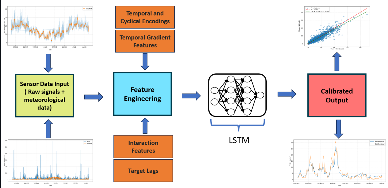
Overview of the calibration methodology: raw sensor data input, feature engineering and preprocessing, LSTM calibration model, and calibrated output.
Dataset and Test Case
The dataset used in this work comes from the OxAria project, a low-cost air-quality sensor network deployed across Oxford, UK. The study focuses on a Praxis Urban sensor co-located with the AURN reference station at Oxford St. Ebbe’s.
The sensor platform measures particulate matter and nitrogen dioxide using:
- an Alphasense NO2-A43F electrochemical sensor for NO2;
- an Alphasense N3 optical particle counter for PM10 and PM2.5;
- meteorological and auxiliary variables such as temperature, relative humidity, sample flow rate, and time-of-flight metrics.
The reference measurements are obtained from regulatory-grade instruments at the co-located AURN site. This co-location is important because both the low-cost sensor and the reference instrument experience the same atmospheric conditions.
The calibration is performed for three pollutants:
- PM2.5;
- PM10;
- NO2.
The data are available at 15-minute resolution, allowing the model to learn short-term pollutant dynamics and sensor response behaviour.
Data Preparation
Low-cost sensors often contain drift, offsets, and short-term artefacts. In this work, the model is trained using baseline-corrected data. This allows the deep-learning framework to focus on temporal calibration rather than raw signal correction.
The cleaned dataset contains pollutant-specific input variables. For NO2, the model uses electrochemical sensor variables such as working and auxiliary electrode voltages. For particulate matter, the model uses variables related to the optical particle counter, such as sample flow rate and sample time of flight.
Temperature and relative humidity are included for all pollutants because they strongly affect low-cost sensor behaviour.
Meteorological and Sensor Signals
The calibration model must account for environmental variability because low-cost sensors respond not only to pollutant concentration, but also to field conditions such as temperature and humidity.
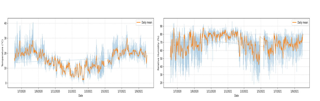
Time series of meteorological variables used in the calibration framework (temperature and relative humidity).
The comparison between raw low-cost sensor signals with the reference are shown in the figure below. This comparison shows the need for a dedicated calibration model, especially when the sensor signal contains peaks, offsets, or drift that do not match the reference instrument.
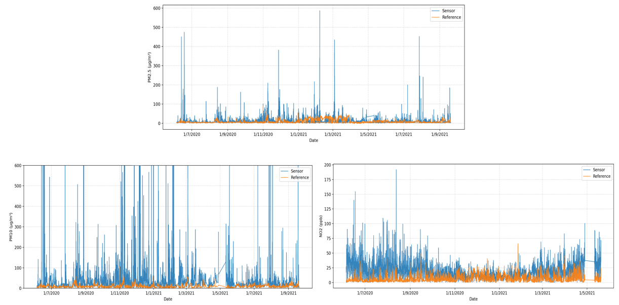
Comparison of low-cost sensor measurements with AURN reference data for PM2.5, PM10, and NO2.
Feature Engineering
The feature set is designed to represent sensor behaviour, environmental effects, and temporal structure. Instead of relying only on the instantaneous sensor reading, the model is given additional information that helps it distinguish true pollution changes from sensor artefacts.
The engineered features include:
- raw sensor values;
- lagged pollutant and meteorological variables;
- short-term percentage changes;
- hour, day, month, and seasonal encodings;
- rush-hour indicators;
- interaction terms between sensor and environmental variables;
- pollutant-specific auxiliary variables.
This feature design allows the model to learn daily cycles, weekly patterns, seasonal effects, delayed environmental responses, and short-term pollutant persistence.
Sequence Construction
The calibration problem is treated as a temporal modelling task. Instead of calibrating each observation independently, the model receives a short history of previous observations and uses that sequence to predict the calibrated concentration at the next time step. This sequence-based structure is central to the framework. It allows the LSTM model to capture persistence in pollutant concentrations, delayed sensor responses, and gradual changes in sensor behaviour.
LSTM Calibration Model
The calibration model is based on a Long Short-Term Memory network. The LSTM receives a fixed-length sequence of engineered features and predicts the calibrated pollutant concentration.
The final model uses:
- a fixed rolling-window input;
- an LSTM layer to capture temporal dependencies;
- a dense layer with nonlinear activation;
- dropout to reduce overfitting;
- a final linear output for calibrated concentration;
- early stopping during training.
The model is trained separately for each pollutant. This pollutant-wise setup is useful because PM2.5, PM10, and NO2 have different sensor responses, noise characteristics, and environmental sensitivities.
Calibration Results
The calibrated predictions are first evaluated using scatter plots against the reference observations. For each pollutant, the calibrated values are compared with the reference values across validation and test datasets. The figure shows the scatter plots for the various pollutants across the test sets.
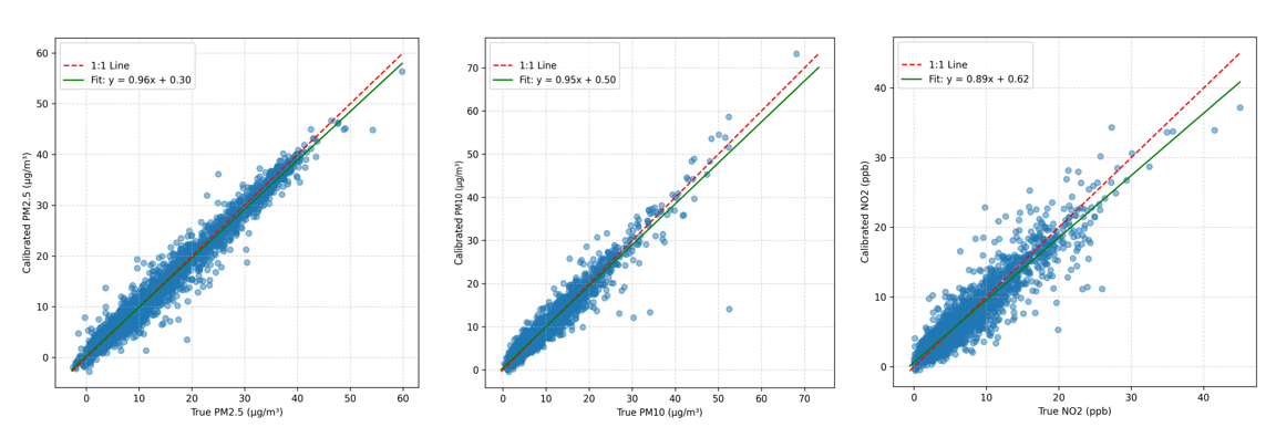
Scatter plots PM2.5, PM10, and NO2 across the test sets. </em>
The scatter plots show that the calibrated predictions follow the reference concentrations closely. PM2.5 gives the strongest performance, followed by PM10. NO2 is more challenging because of stronger short-term variability and traffic-driven fluctuations, but the calibrated output still captures the main concentration patterns.
Performance Metrics
The model is evaluated using R2, MAE, and RMSE. These metrics assess how well the calibrated output agrees with the reference measurement.
The test performance obtained in the study is summarized below:
| Pollutant | Test R2 | Test MAE | Test RMSE |
|---|---|---|---|
| PM2.5 | 0.97 | 0.97 µg/m³ | 1.45 µg/m³ |
| PM10 | 0.91 | 1.16 µg/m³ | 2.07 µg/m³ |
| NO2 | 0.88 | 1.16 ppb | 1.80 ppb |
These results show that the LSTM framework provides strong calibration performance for all three pollutants, with particularly high accuracy for particulate matter.
Generalization to Unseen Data
The trained model is also evaluated on unseen temporal periods that were not used during training, validation, or testing. This is important because a useful calibration model must remain reliable when applied to new field conditions.
For PM2.5 and PM10, the unseen evaluation uses data from 23 to 30 September 2021. For NO2, the unseen evaluation uses data from 23 to 30 May 2021.
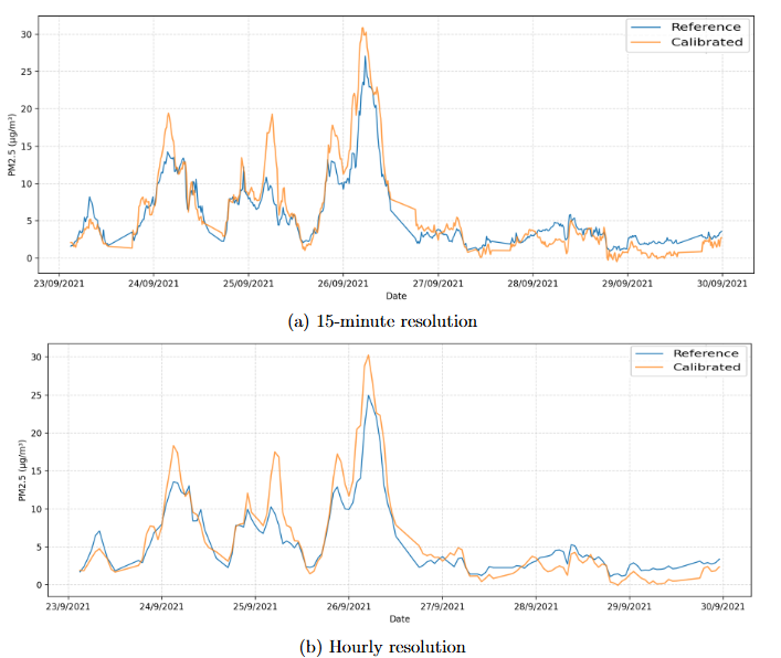
PM2.5 unseen-data calibration results at 15-minute and hourly resolutions.
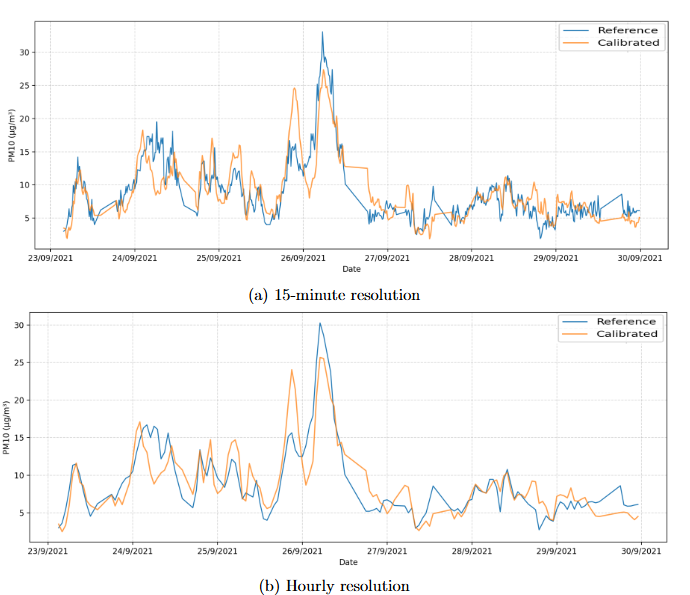
PM10 unseen-data calibration results at 15-minute and hourly resolutions.
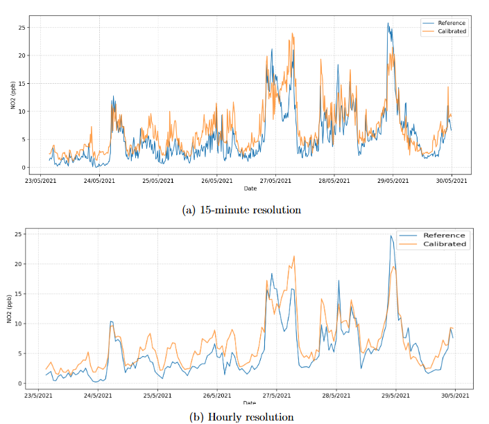
NO2 unseen-data calibration results at 15-minute and hourly resolutions.
The unseen-data results show that the model remains stable under new temporal conditions. Hourly averaging generally improves performance because it reduces short-term noise and makes the comparison with the reference signal smoother.
| Pollutant | Resolution | R2 | MAE | RMSE |
|---|---|---|---|---|
| PM2.5 | 15-min | 0.75 | 1.63 µg/m³ | 2.37 µg/m³ |
| PM2.5 | 1H avg | 0.77 | 1.56 µg/m³ | 2.25 µg/m³ |
| PM10 | 15-min | 0.71 | 2.08 µg/m³ | 2.77 µg/m³ |
| PM10 | 1H avg | 0.74 | 1.90 µg/m³ | 2.53 µg/m³ |
| NO2 | 15-min | 0.63 | 2.21 ppb | 2.86 ppb |
| NO2 | 1H avg | 0.71 | 1.90 ppb | 2.44 ppb |
Regulatory Equivalence Assessment
In addition to standard regression metrics, the calibrated outputs are evaluated using the Equivalence Spreadsheet Tool 3.1. This assessment checks whether the calibrated low-cost sensor output satisfies the uncertainty requirements used for air-quality measurement equivalence.
The expanded uncertainties obtained after LSTM calibration are:
| Pollutant | Expanded uncertainty | Requirement |
|---|---|---|
| NO2 | 22.11% | ≤ 25% |
| PM10 | 12.42% | ≤ 50% |
| PM2.5 | 9.10% | ≤ 50% |
These results show that the calibrated low-cost sensor measurements satisfy the required data-quality objectives for objective air-quality estimation.
Applications
This calibration framework can support:
- correction of PM2.5, PM10, and NO2 low-cost sensor measurements;
- dense urban air-quality monitoring networks;
- sensor-informed pollution mapping;
- long-term low-cost sensor deployment;
- quality improvement of environmental sensor datasets;
- real-time or near-real-time air-quality analysis;
- integration of calibrated sensors into digital-twin workflows;
- regulatory screening and objective estimation studies.
Code and Data Availability
-
Tutorial: Low-cost sensor calibration tutorial